AutoFickle

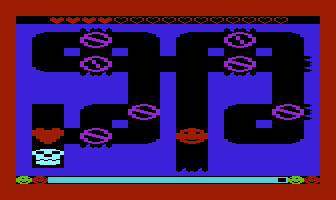
Fickle is a one-button Vic20 game written by my friend Malcolm Tyrrell. In it, you steer a character called Fickle through a maze, trying to reach a heart. Your control is limited to choosing (by pressing a key) whether Fickle obeys or ignores various objects in the game.

After having good fun playing it for a while on the xvic emulator (part of the Vice project), I thought it would be interesting to write a program which runs alongside the emulator and automatically plays Fickle, by watching the screen, looking at the levels, working out what to do, and pressing a key at the right times.

The idea sat for a while, until I eventually got round to it. It was an interesting project, and was successful — AutoFickle plays the entire set of fifteen levels straight through:

(The video has been post-processed to add the ‘subtitles’, but apart from that it’s a faithful recording of what you see on the emulator while AutoFickle’s playing the game.)

In this post I give an outline of what was involved and how the pieces work and fit together.

What is Fickle?

The best way to get a feel for the game is to play it. It can be found at Malcolm’s Projects page; you’ll also need the relevant emulator for your platform from the Vice pages.

The rules are explained by Malcolm in a post on the Denial forum:

Fickle has two states: “Do” (green) and “Don’t” (red). The only control you have (any key except Restore) is to toggle between these states.

When in the “Do” state, passing over a floor tile will have some effect:

• clockwise/anticlockwise tiles turn Fickle left/right
• Fickle picks up the heart, keys, etc.

On the other hand, tiles are ignored in the “Don’t” state.

One other point might be worth emphasising: the state only affects floor tiles and not doors or barriers (as occur in later levels).

I give a bit more detail on the effects of each game element in the do/don’t states below.

Connecting the emulator to AutoFickle

The first step is to allow a program to ‘watch’ what’s happening on the emulated TV screen, and ‘press keys’ when required. I wrote an addition to xvic to allow this. It consist of a fake graphics driver which dumps screenshots to a ring buffer in Posix shared memory. It then uses a Posix semaphore to notify clients when a new screenshot has been dumped into the buffer. On the client (i.e., AutoFickle) side, I wrote a small piece of C++ to handle the semaphore; AutoFickle itself is written in Python, which ‘mmap’s the actual screenshot objects directly.

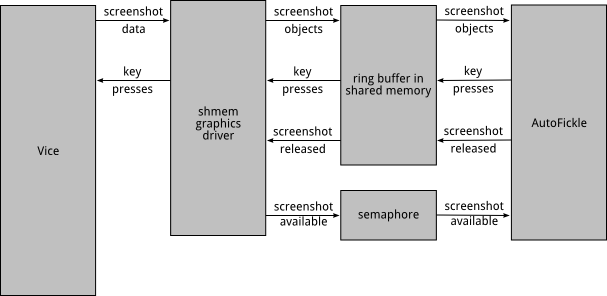
When the client releases each screenshot back to the ring buffer, it can optionally request a keypress be sent to the emulator. This is what allows AutoFickle to ‘press a key’ in the game. It’s probably a bit of a stretch for a graphics driver to be pressing keys, but it works.

Identifying the map

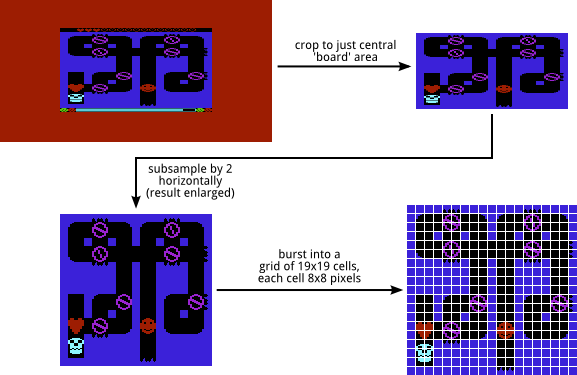
Once AutoFickle is receiving the screenshots, the first task for the program is to identify the map of the level. We’re aiming for a high-level description along the lines of ‘the heart is at (8, 8); an anticlockwise spinner is at (3, 4); the skull floats back and forth between (1, 1) and (4, 1)’.

The process starts by cropping the screenshot down to just the central ‘board’ region. It then subsamples by a factor of two horizontally — xvic doubles each pixel to give a better impression of the original aspect ratio, and we wish to undo this. We then exploit the fact that the game board is a 19×19 grid of ‘cells’, where each cell is 8×8 pixels.

From bitmaps to glyphs

We now want to identify the contents of each cell. AutoFickle flattens each 8×8 cell into a 64-element vector of palette entries. It then attempts to look up each such vector in a dictionary, which gives it a label such as ‘spike-d’, to indicate a cell containing spikes pointing downwards. At this point we know which ‘glyph’ is in each cell; a glyph is a name for a particular 8×8 pattern of pixels. To build the dictionary, I started by semi-automatically identifying common patterns in the screenshots, then manually labelling them. About half way through I instead used the source code which Malcolm provides, convincing myself that this wasn’t cheating as I had demonstrated that the fully-clean approach did work.

Sometimes there are unknown 8×8 blocks, so there’s a voting mechanism whereby a cell has to be identified as a particular glyph several times before the conclusion is firm. For some cells, this doesn’t work. The electrified barrier is essentially random so there’s a fudge to look for otherwise-unidentified blocks of ‘barrier colour’. The skull is dealt with separately (see below).

This is quite CPU intensive, but my (fairly old) machine keeps up. Some example glyphs:

spike-d	corner-bl	spinner-tr-2
(spikes pointing down)	(bottom-left corner in corridor)	(top-right quarter of spinner, phase 2)

From glyphs to map elements

We then want to identify the higher-level ‘map elements’ of the level, by context (spatial and temporal).

Spatial context allows us to resolve situations like the following: the top-left and top-right quarters of the heart are the same glyph, but we can tell which map element is which by what’s to the left and right of, and above and below, each. Continuing with the heart as an example, the whole process is:

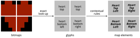
The contextual rule used here for the top-left quarter is ‘I am glyph heart-top, below me is heart-bl, to the right of me is heart-top; therefore I am Heart-Top-Left‘, and similarly for the other quarters.

Temporal context similarly allows us to resolve spinner direction, by comparing one frame to the next, on frames where the glyph changes. From a single image, we can label a spinner corner as belonging to a particular one of the four ‘phases’, and then depending on whether those phases go 0,1,2,3 or 0,3,2,1 as time marches on, we can tell whether it’s spinning clockwise or anticlockwise.

The skull

The skull required special handling. To avoid having to have glyphs for every frame of the skull’s animation, the code looks for cells containing enough ‘skull colour’. The skull is the only thing of its colour, so this fudge works.

AutoFickle builds up a list of cells where the skull has been seen, and once it has a list consisting of two copies of the same half, it concludes that one such half is the full cycle of the skull’s movement.

Level simulation

Once it has the level in terms of map elements, the code can simulate how the level would play, noting what happens when Fickle makes a choice between “do” and “don’t”. It has to keep track of all relevant information about the game, which it bundles into a Game State object:

• Fickle’s pose (location, and direction of travel);
• Which keys have been collected, and which doors opened;
• The state (open/closed/electrified) of any barriers;
• The phase of the skull in its cycle (in whole and 1/3 steps).

Each game ‘tick’ then causes a transition from the ‘current’ Game State to the ‘new’ Game State(s). Very often there is only one successor, because Fickle just moves one step in his current movement direction. Only when Fickle makes a choice (by being “do”/”don’t”) are there two. In this way, we can build up a graph of the level, where each node is a Game State. An example is below.

In building this graph, we have to handle:

Initially: Graph nodes are Game State objects

An extract from an example such graph, showing how most nodes have exactly one successor, but where Fickle’s “do”/”don’t” state makes a difference, there are two:

(The spinner here is spinning anti-clockwise.)

The starting node of the whole graph has just one successor, except when the level contains a skull. Then we enter a different Game State depending on where the skull is when we launch Fickle. To capture this, we generate one Game State per possible phase of the skull, and process all of them. In earlier versions of the code, I tried to economise by only allowing integer skull starting phases, but AutoFickle failed to solve one level until I allowed it to time its start more carefully by allowing ‘thirds’ in the skull phase too.

Transform to: Graph nodes are Game State Run objects

To make the graph easier to visualise, and also to speed up future processing, we collapse ‘runs’ of Game States into single nodes in a new graph. We absorb any single-predecessor, single-successor node into its predecessor, to get runs of Game States. Within a run, the Game States inevitably follow one from another. We then have a graph whose nodes are ‘Game State Run’s. In this excerpt, only the relevant section of the map is shown:

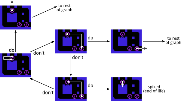
The loop in the lower-left corner of this graph represents the situation where Fickle is bouncing back and forth in the “don’t” state.

Solving the level

Using the ‘collapsed’ graph of the level, we can now find the shortest path from the start node to the winning node, i.e., a Game State where Fickle is on top of the heart. The code uses Dijkstra’s algorithm, with the naive ‘search for minimum each time’ approach. This gets a bit slow for complex levels, but all levels are solved within the time limit, so there was no need to do anything cleverer.

The length of an edge is the number of Game States in the source node. This gives a minimally-quick route through the level, measured from the time we launch Fickle. When there’s a skull, it sometimes does mildly counter-intuitive wiggles to get the skull phase right for later in the level. On one level, it toggles a switch twice rather than leaving it alone; this makes no difference in the time taken, so it’s an essentially arbitrary choice between toggle zero times or two times.

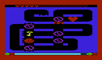
We take the level shown on the right as an example. It has a key, a door through which Fickle must pass, and various spinners and spikes.

In the graph, there are four sets of spikes upon which Fickle might become impaled. Each black dot is a run of Game States which follow one to another; Fickle starts at the left-most node. The shortest winning route, to the heart, is shown by the thick arrows. Red arrows are when Fickle is in “don’t” state; green arrows are “do”; black arrows are for an inevitable progression between nodes.

This graph has 37 nodes; levels with a skull have many more nodes, arising from the inclusion of the skull-phase in the Game State. The most complex level by this metric is level 10, with 1451 nodes — it includes a skull and switched barriers.

Creating a plan of action

The winning path through the graph translates into a description of which game elements (spinners, switches, keys) we must “do” and which we must “don’t” when Fickle passes over them. The required state is represented above by the colour of the edge by which we leave a node. We also know that we start in the “do” state, and must land on the heart while in the “do” state. If a “do”/”don’t” requirement is different from the previous one, AutoFickle must request a keypress between the two, to toggle Fickle’s state:

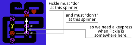
The animation is not quite predictable enough to just play blindly based on counting frames. So the level-solving code creates a set of ‘Fickle checkpoints’, having Fickle’s location and direction for each Game State Run in the winning path. At some checkpoints, AutoFickle presses a key, as in the example above. There is a tolerance of a few pixels in deciding when Fickle has reached the checkpoint.

Tracking Fickle

We can exhaustively search the full screenshot for Fickle, but this is slow, so we cannot do this on every frame. So we predict where Fickle is going to be, using a simple model: he keeps going in the same direction. We then search only in a small area around that location, and we can exploit the knowledge that at least one of Fickle’s coordinates is a multiple of 8. If he bounces off a wall or diverts round a corner, we find him by this method. If we do not find him, we fall back to a full search of the screenshot. This happens when Fickle tears (rare, and then we find him next frame), or when Fickle teleports. The ring buffer allows us to catch up to real-time again once we’ve found him.

Other types of checkpoint

There are other types of checkpoint. One allows us to wait for the skull to reach a particular phase in its cycle (which takes two skull locations, to make sure it’s travelling in the required direction). Another gives a delay of one frame, for precise setting of Fickle’s launch-time compared to the skull phase.

Putting it all together

AutoFickle starts in the map-identification stage, then constructs the graph, finds the shortest route, and builds its plan of action. It carries it out, by watching for checkpoints and sending keypresses where required. Fickle then reaches the heart, a new level appears, and the process begins again.

Success!

Conclusions

As I wrote AutoFickle, there were several points where I had to write more code, or correct existing code. But there were many levels which AutoFickle solved completely unseen; this was gratifying. There is no level-specific knowledge encoded in AutoFickle.

Python was a good language to work in, given that it turned out to be quick enough. I structured the code so that I could record sequences of screenshots to Python pickles in files, and play them back, to avoid having to fire up the full emulator each time. This was a big help to development.

When discussing the project with Malcolm, he pointed out the fact that’s the level maps are really built on a 6×6 grid of 2×2 cells, with 1-cell ‘gutters’ between. Had I noticed this myself, it might have simplified the map-identification stage.

It might be interesting to pick path with the greatest ‘margin of error’ for skull-avoidance. We could examine the (say) ten shortest paths, and look at the closest Fickle gets to the skull in each one. The chosen route would then be the one with the largest such ‘minimum skull clearance’ value.

I decided that I would be content to take advantage of particular features of how Fickle worked. In other words, I would not try to solve some fully general sub-problem where doing so would turn into a project in its own right. This sometimes required a bit of self-discipline, but kept the scope of this fun project finite.