A game of multiples and divisors

One of the projects at the Young Scientist exhibition in mid-January 2015 was an interesting number-based game implemented in Scratch. It won third prize in the ‘junior group’ category.

This post presents the game in a different format, and develops a computer player for it.

Embarrassing confession

I did the analysis based on my memory of the game from visiting the exhibition. I only thought to check whether the Scratch project was public at the final stages of putting this post together, when I discovered the Scratch game was public, and that I had slightly mis-remembered the rules. The approach described below applies perfectly well to the real game, but the conclusions are different. The results (and computer player) for the real game are given at the end.

The game (as I mis-remembered it)

Players take turns to choose a number greater than 1 but less than 100. On each turn, the player must either choose a multiple of the other player’s previous choice, or a divisor of it. You are not allowed to choose a number which has already been chosen (by either player) earlier in the game. If a player has no numbers to choose from, because they’ve all been chosen already, then that player loses.

The first turn is special — you choose any number greater than 1 but less than 50. This avoids a trivial game whereby the first player could immediately win by choosing a prime over 50.

In the version below, you play against the computer. You choose a number by clicking on it: your choices are shown in red. The computer then responds: its choices are shown in blue, and it highlights then plays one of them. Your new choices are then shown in red, and so on.

You play first:

Initial analysis attempts

This is a deterministic game with perfect information, so theoretically it is either a win for the first player or for the second.

I guessed that some thought might reveal a winning strategy, but I failed to come up with anything. A few small observations did occur to me: a game which has so far evolved as ’10’, ’40’, ’20’, ’80’ is equivalent to one which has evolved as ’10’, ’20’, ’40’, ’80’; it is impossible for a prime greater than 50 to ever be played; thinking of the numbers as their product-of-primes representation suggested that the game took place on a multi-dimensional ‘cube’ of prime powers with many corners chopped off. But nothing which solved the problem.

It is certainly possible that more thought would yield the answer, but I decided to try a different approach.

Brute force

We can think of the possible ways the game can evolve as a ‘game tree’. In this representation, a node stands for a state of the game, and an edge stands for a move which turns one game-state into another. Call a node a ‘winner’ if the player whose turn it is to move from the game-state represented by that node can definitely win if they play correctly. Equivalently, a node is a ‘loser’ if the player whose turn it is to move from that state is definitely going to lose no matter what they choose. Then we can express the rule for deciding whether a node is a winner as:

A node is a winner if and only if at least one of its children is a loser.

(In other words, the player choosing which move to make from a particular state of the game can win if and only if there is at least one move they can choose which makes the other player have to play from a ‘losing’ state.)

This formulation correctly captures the case that a node with no children is a loser — if a node has no children, then there are no possible moves from that node, and such a state means the player whose turn it is to move has lost.

In our case, it is easy enough to work out at each node what its children are, by keeping track of the essential game state (most recent number played; which numbers have been played so far).

On running an initial attempt to code this, it was obviously going to take infeasibly long to get anywhere. A multi-day run had made very little progress; it was still considering games where the first player played ‘2’.

Choosing which children to explore first

Consider a piece of game tree like this:

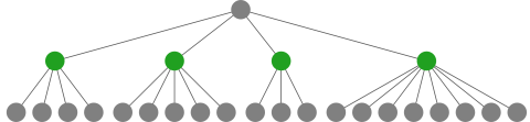
(Unfortunately, common practice is to draw the ‘root’ at the top of the diagram, which is upside-down compared to a real tree.) The green nodes will be referred to below.

We are trying to determine whether the top (root) node is a winner or loser. Recall the rule:

A node is a winner if and only if at least one of its children is a loser.

If we examine the four green children of the root node one at a time, we can stop as soon as we find a ‘loser’ child. How do we know if a green node is a loser? By re-phrasing the rule, we see that this happens if all of its children are winners. In very woolly terms, it seemed plausible that if we examine a green node with a small number of children, we’re more likely to discover that they’re all winners, and so conclude that the green node is a loser, and so conclude that the top (root) node is a winner. In the example, we might be better off studying the third green node (with its three children) first. Importantly, changing the order in which we examine a node’s children does not affect the correctness of the answer we reach.

This is certainly very fluffy ‘reasoning’, but an approximation to it turned out to do the trick:

To avoid re-computing a list of multiples and divisors at each move, the analysis program stores a table of lists, one for each number between 1 and 100. Some examples of these ‘possible responses’ lists are:

3 :	6, 9, 12, 15, 18, 21, 24, 27, 30, 33, 36, 39, 42, 45, 48, 51, 54, 57, 60, 63, 66, 69, 72, 75, 78, 81, 84, 87, 90, 93, 96, 99
5 :	10, 15, 20, 25, 30, 35, 40, 45, 50, 55, 60, 65, 70, 75, 80, 85, 90, 95
15 :	3, 5, 30, 45, 60, 75, 90
30 :	2, 3, 5, 6, 10, 15, 60, 90
45 :	3, 5, 9, 15, 90
60 :	2, 3, 4, 5, 6, 10, 12, 15, 20, 30
75 :	3, 5, 15, 25
90 :	2, 3, 5, 6, 9, 10, 15, 18, 30, 45

To implement the ‘examine children leading to fewer grandchildren first’ idea, we sort each ‘possible responses’ list such that entries having fewer ‘possible responses’ come before entries having more ‘possible responses’. This sorting is static and need be done only once — it takes no notice of what’s already been played. In the example above, we would re-order the list of possible responses to ’15’ as

15 :	75, 45, 30, 60, 90, 5, 3

because ’75’ has only 4 possible responses, ’45’ has 5, and so on up to ‘3’ which has 32.

Conclusion: the second player can always win

With this change, the program arrived in reasonable run-time at the result:

The game is a loss for the first player.

This is why the human goes first in the implementation at the top of this post.

Construction of a computer player

The next job was to make a computer player for the game. Setting the human up as the first player will mean that the computer will always win. There were then a few engineering points to take care of.

The full game tree is very large. We can first note that we do not need to store all children of a winning node, only the first-found of its losing children. Even with this saving, we get a tree with 282 million nodes. This is too large to sensibly store in a web page.

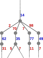
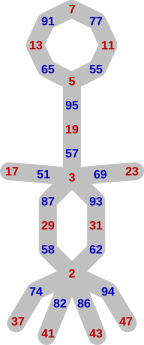
If we look at a small subtree, we observe lots of redundancy as the games finish. In the illustration of the end of a game on the left here, we only show the moves made as the game progresses. To clarify this representation, the start of the subtree is shown fully on the right, with the nodes, and with the moves labelling the edges.

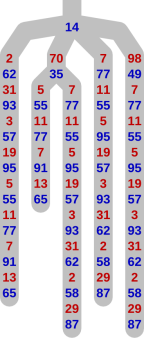
The chain of moves ‘7, 77, 11, 55, 5, 95, 19, 57, 3, 93, 31, 62, 2, 58, 29, 87’ occurs three times here. (At the end of that chain, the blue player wins, because the only factors of 87 are 29 and 3, both of which have already been played.) The chain ‘5, 55, 11, 77, 7, 91, 13, 65’ occurs twice. In a larger tree the redundancy is greater.

From the point of view of using this tree to drive a computer player’s behaviour, we can unify each set of ‘equivalent’ subtrees, and store the information once only. Under this scheme, the above example would become

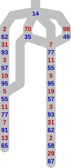
It doesn’t matter if the game has evolved differently before the point where paths converge, as long as the behaviour from that point onwards is identical. This happens if the winner’s responses are the same, and the loser has the same list of choices at each turn — that is what we mean by ‘equivalent’.

Performing this unification is a special case of the problem known as ‘Frequent Subtree Mining’. Our tree is small enough that we can be fairly simple-minded about it. We use the ‘depth-first canonical string’ (DFCS) of the subtree rooted at each node to identify it. We build a map from DFCS to the unique representation of such a subtree. Starting with the deepest node, we check whether the DFCS of the subtree rooted at each node is already in the map. If it isn’t, we insert into the map a copy of the node, replacing its children with references to their representations already in the map.

Most of the savings come from unifying the most common subtrees: 1% of graph nodes represent more than 98% of the tree nodes.

Because of RAM limitations, the approach was in fact to create one game tree per initial move of the human player, and turn that into a unique-ified graph.

Instruction tables

Once we have a ‘unique-ified’ graph, we must represent it in a way which allows the computer to play the game. We do this by constructing an ‘instruction table’ for a simple machine. Each entry in the table represents a winning node and its losing children, linking in turn to their winning children. This extract illustrates the idea:

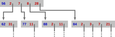
When playing as the winning player, the top instruction represents the situation where we have just played ’56’ and are awaiting the opponent’s response. The numbers 4 and 14 have already been played. When the opponent chooses their move, we follow the matching arrow, and our response is contained in the instruction we arrive at. In this example: If the opponent chooses 2, we play 62 (and await their next move, which in fact must be 31); if 7, we play 77 (and wait for them to play 11, their only option); if 8, we play 88 (and wait for them to choose between 2 and 11 — this extract describes a game where 4, 22, and 44 have already been played); otherwise the opponent’s move must be 28 and we play 84 (and wait for them to choose between 2, 3, 7, and 21 — this extract describes a game where the other factors of 84 have already been played).

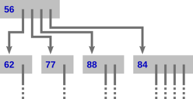
We can compress the representation by noting that at each point in a game, we know the set of possible moves the human will choose from, and can sort them in increasing order, as above. Therefore, we need not store this information in the instruction. By eliminating this redundancy, the instruction table only has blue numbers and pointers, and the extract looks like

Finally, we pack the entries into a flat array, where arrows are indexes into the same array, and the blue moves are stored as-is. This requires a two-pass process, because the entries are of varying size: first, calculate offsets of each winning node’s entry; second, populate the entries now that each node’s location in the array is known.

Instruction table ‘overlays’

Alas, the biggest such instruction table (handling the case where the human player starts with 45) was 638KB in size, which seemed an uncomfortably big download.

To address this, we chop the original game tree at various prune/graft points. The instruction table entry for such a graft point will have a special form meaning ‘request more instructions’. This request is made by referring to the node in the tree by the list of moves played to reach it.

We find suitable ‘prune points’ by trying to find subtrees with between 300k and 500k nodes (choosing those bounds by rough experiment) and then unique-ifying and translating to instruction tables. This gave 1111 instruction sub-tables, of median size 7KB. The largest is 18KB, and the smallest is 14 bytes. Ideally this range would be tighter, but a complete solution was looking difficult, and the set of 1111 files is not disastrous.

Testing and statistics

To test this instruction-table overlay machinery, a program written in C++ simulates random human play, emulating the process of overlay loading with an in-memory vector of tables, populated on demand from the same files used in the Javascript version in this post. For each simulated game, it performs some validity checks:

• the computer always wins;
• the instruction table never fails (no arrows point beyond the end of the table);
• the computer never plays a number not among its valid choices.

This test process played a billion games with no faults in around half an hour.

As a side-effect of the testing process, we have the following distribution of game length:

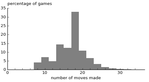
Only even-length games are possible, because the computer always wins. The distribution is not straightforward, and there is a very thin tail out beyond the range shown in this graph. The longest game randomly found during testing was of 56 moves.

We can also look at the distribution of how many overlay requests were made:

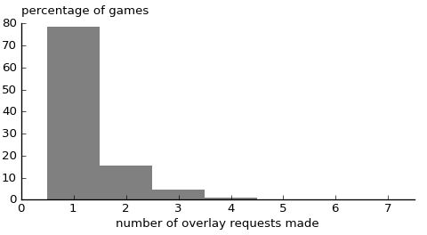
No game required more than seven requests. It is unusual to require more than three overlay requests; this happens around 1.2% of the time.

Javascript implementation

Finally, I wrote the Javascript version used in this post. This was fairly straightforward, using jQuery. A concept new to me was the use of Javascript ‘promises’, which represent a computation which will in due course yield an answer. This allows tidier expression of asynchronous behaviour. In particular, the logic for launching a request for the next instruction table overlay chunk (when required), while proceeding with the rest of the behaviour, came out quite cleanly. The flashing colours provide a bit of time for the server to respond.

The program starts with a ‘bootstrap’ instruction table, constructed from a hard-coded list of responses to the human’s first moves, each labelled as a prune/graft point. Beyond that, the overlay request mechanism takes over.

If you click on the disabled ‘1’ cell, the delays are reduced to 1/100 of their normal length, allowing more rapid play.

Analysis of end-game

Eventually the human is forced into playing a prime less than 50. From that point, play evolves along the paths in the graph to the right. The computer chases the human into one of the loops and then wins.

Possible future work

• The analysis and pre-processing was all done using C++11. Ideally I would make the code available, if I get the chance to tidy it up. It might be a good experiment in using git to explain the development of a piece of code.
• There are several tiny instruction sub-tables. If the human player starts with a prime number, the game is very short, as noted above. It would be good to subsume all these tiny sub-tables into the bootstrap table.
• It might be possible to compress linear ‘chains’ of instruction table entries into some more compact representation.
• What is the longest game under this computer strategy?
• The computer does not play optimally, in the sense that it sometimes could force a win more quickly. (E.g., if the human starts ‘7’, the computer does not simply chase them round the 7–77–11–55–5–65–13–91 loop.) More generally, how much of the above behaviour is dependent on the strategy used to search for winning moves?
• Extract a higher-level description of optimal play, at the level of ‘force the other play to play a prime’.
• Generalise to other graphs: in this setting, the game is to move a rubber stamp from node to adjacent node, where already-stamped nodes are disallowed.

The original game

As confessed at the start of this post, the real game has a small but important difference from the one described above.

The real game has inclusive upper bounds for the numbers the players may choose. I.e., ’50’ is a valid choice for the first player, and ‘100’ can be a valid choice thereafter. The Scratch project allows ‘1’ as a valid first move but not subsequent move. I’m sure I remember the student explaining that ‘1’ was not permitted (at all). Also, the Scratch project says as part of its documentation

Then at the first go enter a number between 1–50 (set at 50 at the first go to give a chance to the other player to compete).

This ‘give a chance to the other player’ remark suggests the ‘disallow 1’ interpretation is correct. Therefore we continue to forbid ‘1’ in this re-done analysis.

With this set-up, repeating the above work revealed a different conclusion:

The first player can always win, by starting with ’50’.

(It’s possible that other first moves will also give a win to the first player. I haven’t done the full analysis.) Here, the computer has played ’50’ as its first move, and you, futilely, play next:

Edit

Thanks to Adam Spiers for suggesting that I give more detail in the explanation of a ‘game tree’ and the ‘node is a winner if and only if at least one of its children is a loser’ rule. [20150428]